
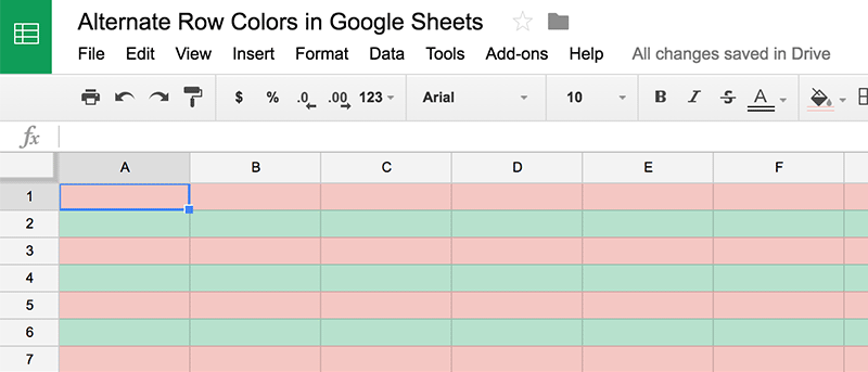

Google Sheets is a great way to create spreadsheets online, and it comes with tons of features to make your life easier. For instance, it lets you create spreadsheets that you can share with others, apply formulas, add styling, and do tons of other things.
While it has all the formatting tools to help you format your sheets, the one thing that I did not find in it was the feature that lets you apply alternate row colors. That way you can have a color for an even row and then another color for the odd row. It is something that helps you make reading spreadsheets easier, and it also helps the sheets to look good in terms of appearance.
Since the feature is not available by default, you might think it is not possible. But wait – you do have a way to do it using conditional formatting and a couple of formulas.
Alternate Row Colors in Google Sheets
1. Open a web browser on your computer and head over to the Google Sheets website. Log in to your Google account if you are not already logged in.
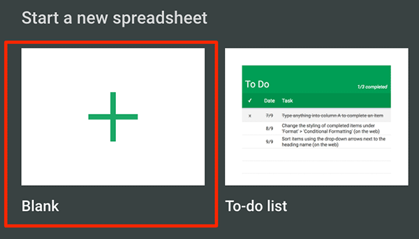
Once you have logged in, create a new spreadsheet by clicking on “Blank” in the “Start a new spreadsheet” section. It will create a new spreadsheet in your Google account.
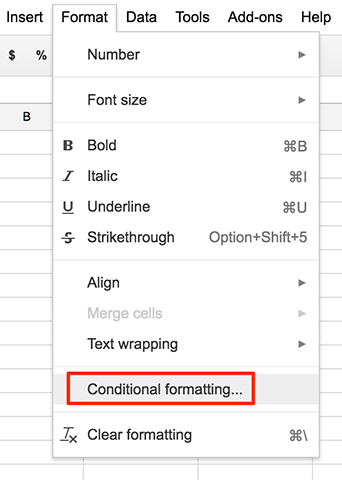
2. When the new blank spreadsheet opens, click on the “Format” menu on the top and select the option that says “Conditional formatting…” as shown below. It will apply the formatting depending on the given conditions of your spreadsheet.
3. A new panel should open in the right-hand side with the title “Conditional format rules.” Here you need to specify the conditions for the formatting that you are going to apply to your spreadsheet.
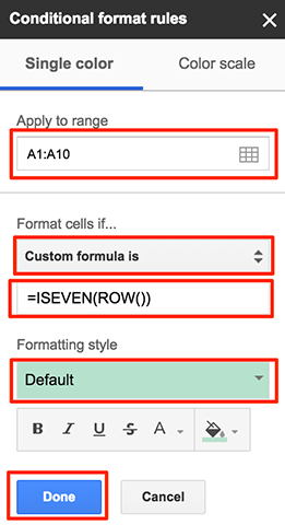
You should enter the following details in the input boxes:
Apply to range – choose the cells where you wish to apply the alternate row colors. Click on it and it should let you select the cells in the spreadsheet, or you can manually enter the values.
Format cells if – this option lets you choose when the specified cells should be formatted with your chosen formatting settings. From the given drop-down menu select the “Custom formula is” option.
Value or formula – enter =ISEVEN(ROW()) in this field. It tells the spreadsheet to only apply the chosen formatting when the row is even.
Formatting style – select the style of formatting that you would like to apply to the cells. You can leave it to the default if you do not want to change it.
Click on “Done” at the bottom to save the settings.
4. You should now be able to see the specified formatting applied on the cells in the spreadsheet.
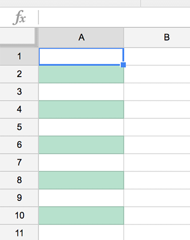
5. You have successfully applied the chosen color to the even rows and and now need to do it for the odd rows. For that click on “Add another rule” in the same panel you have in the right side of your screen, and it will now let you add another rule for conditional formatting.
6. Once again the same settings boxes will appear for you to fill in. This time what you need to change is the formula and the style as shown below.
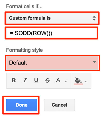
Custom formula – Type in =ISODD(ROW()) and it will only apply the chosen settings to the odd rows in the spreadsheet.
Formatting style – choose a color that you wish to apply to the odd rows in your spreadsheet. Make sure to choose a different color than what you chose above, or it will all look the same.
Click on “Done” to save the rule.
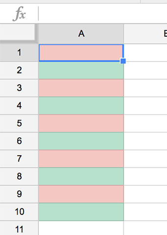
7. The result should be instant, and the following is what it looks like in my case.
Conclusion
If you wish to have style and make reading your spreadsheets easier, you can use alternate row colors in Google Sheets as shown above.
Let us know what color combination you used for your sheets!